Resolution Selection

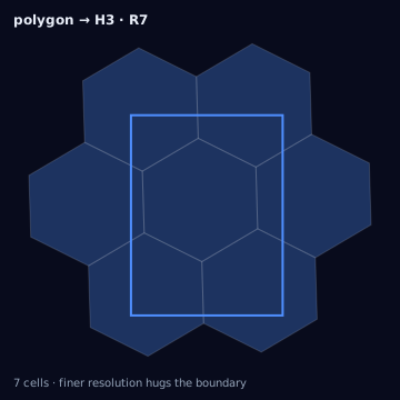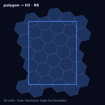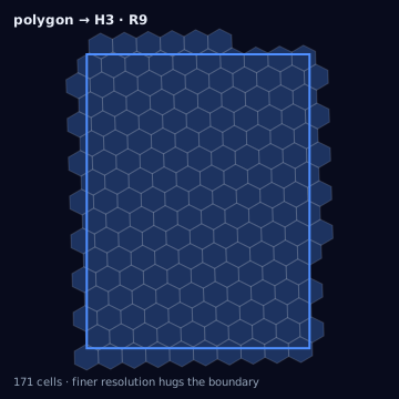
H3 resolution is not a single knob tuned for "accuracy." It sits at the intersection of at least twelve independent constraints, several of which push in opposite directions. A resolution chosen for boundary fidelity can violate a platform's target-count limit; a resolution chosen to satisfy a privacy threshold can be too coarse for the experimental unit it needs to support. This page is a decision guide, not a lookup table — the profiles at the end are defaults for common intents, not universal truths.

The reference table

Each step up in H3 resolution shrinks average cell edge length by roughly a factor of 2.6 and average cell area by roughly a factor of 7 (approximate values, per the h3geo.org resolution table):

Res 5

~252.9 km2 avg area, ~8.5 km avg edge length

Res 6

~36.1 km2 avg area, ~3.2 km avg edge length

Res 7

~5.16 km2 avg area, ~1.2 km avg edge length

Res 8

~0.737 km2 avg area, ~0.46 km avg edge length

Res 9

~0.105 km2 avg area, ~0.17 km avg edge length

These are averages over all cells at a resolution, not a per-cell guarantee: individual cells vary in area and edge length depending on their position relative to the icosahedron (see pentagons and face-crossing distortion), and the variance grows at coarser resolutions. Treat the table as an order-of-magnitude guide for planning, not as a per-cell specification.

The twelve constraints

Geometry size and boundary complexity. A resolution should be fine enough that the source polygon's boundary is not dominated by a handful of cells — a jagged coastline or a county line with many inflections needs a finer resolution than a smooth ellipse of the same area to keep boundary-disagreement area small relative to total area.

Coordinate accuracy. Resolution finer than the source coordinate precision is false precision. A bidstream ping rounded to two decimal degrees (roughly 1.1 km of latitude error) cannot support resolution 9 (edge ~170 m) — cap the effective resolution to the coordinate's actual precision, not its nominal one.

Audience or inventory density. Sparse-audience geographies need coarser cells to accumulate enough observations per cell to be statistically or privacy-meaningfully non-zero; dense urban geographies can support finer cells without emptying most of them.

Platform minimum radius. If execution will be a point+radius circle, the inscribed or circumscribed radius at the chosen resolution must clear the platform's minimum-radius floor — resolution 9 cells are frequently too small to produce a radius any DSP will accept, forcing a coarser resolution regardless of boundary fidelity.

Target-count limits. Platforms cap the number of discrete targets per line item. A fine resolution over a large area can produce an inventory of cells that exceeds the cap before compaction; see platform target-count constraints.

Privacy threshold. A resolution fine enough to isolate a household violates k-anonymity norms; privacy-safe profiles enforce both a minimum physical cell size and a minimum audience count per reported cell, and will coarsen resolution specifically to clear that floor.

Experimental unit. Geo-experiments need units small enough to allow many independent replicates but large enough that adjacent units do not leak treatment into control through normal population movement — usually a coarser resolution (5-7) with a buffer (inscribed circles or gaps) rather than the finest resolution available.

Reporting granularity. If the downstream report only breaks out by state or DMA, executing at resolution 9 buys precision that is destroyed at the reporting join — resolution should match the coarsest mandatory reporting join in the pipeline, not exceed it for no visible benefit.

Computation cost. Cell count grows roughly sevenfold per resolution step; polyfilling, crosswalking, and metric computation over a country-scale polygon at resolution 9 is a materially larger job than the same polygon at resolution 6, with cost that compounds across every downstream join.

Population density variance. A single fixed resolution over both dense urban cores and sparse rural areas will over-fragment the city and under-resolve the countryside; this is the core argument for mixed resolutions rather than one resolution for an entire geography.

Crosswalk stability. Finer resolutions produce more cells per admin region, each with a smaller intersection fraction, which is more sensitive to boundary vintage drift — a crosswalk built for long-term stability should favor a coarser resolution even if a finer one is available.

Expected inventory. The number of cells actually available for targeting or measurement after compaction and platform constraints is the real deliverable; resolution choice should be checked against expected post-compaction inventory, not against the pre-compaction cell count.

Recommended profiles — not universal truths

Admin partition / reporting rollup

Res 7-8: fine enough to track county/DMA boundaries, coarse enough to keep crosswalks stable and inventory manageable.

Store trade-area / proximity targeting

Res 8-9: fine enough to resolve individual retail catchments; verify against platform minimum radius before committing.

Geo-experiment treatment/control

Res 5-7 with inscribed-circle buffering: coarser units reduce control contamination even at some cost to replicate count.

Privacy-constrained audience reporting

Res 6-7, degraded further per-cell if the audience threshold is not met: resolution is a privacy control here, not a fidelity control.

National-scale planning / DMA-only platforms

Res 4-5: matches city/DMA grain; finer resolution buys nothing a DMA-level platform can express.

Edge cases

Mixed-resolution sets (mixed-resolutions) arise naturally when different regions of one target need different resolutions for density reasons; they must be normalized to a common resolution before set operations, never compared as-is. A platform's minimum-radius floor (minimum-radius) can force a coarser resolution than boundary fidelity alone would choose. Tiny polygons smaller than a single cell at the chosen resolution may receive zero center-contained cells regardless of how important the target is — resolution selection for small trade areas should be checked against the source polygon's actual area, not assumed from a profile.

Illustration — the same square at three resolutions